Interactive Apps

The Interactive Apps dropdown from the toolbar will list a few standalone programs you are able to launch directly from the browser as well as an HPC Desktop that will allow you access all of the other software on Cheaha.

Currently, the available standalone programs are IGV, Matlab, RStudio, SAS, and Jupyter.

All of the interactive apps have similar setup pages. For instance, if we click HPC Desktop, the following screen will appear:

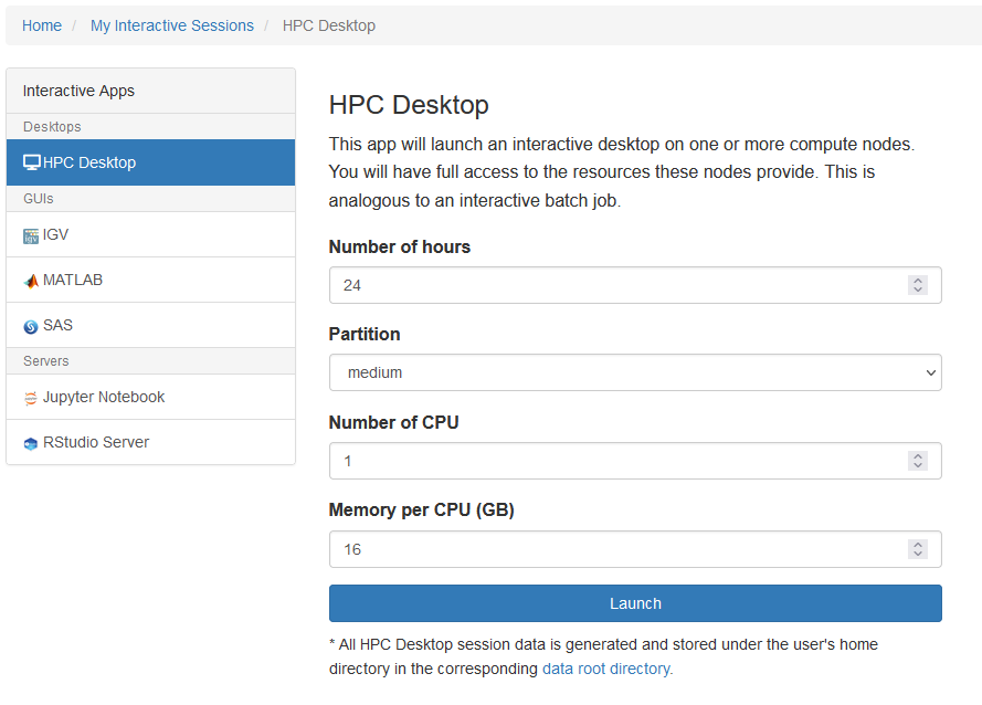
This will allow to choose the number of hours, partition, number of cpus, and memory per cpu needed for the job. These fields are common to all interactive apps and are required. Not all partitions are availabe when creating an interactive job in OOD. For instance, if you need to use the largemem partition, request those resources in a terminal session for an interactive job or submit a batch job.

Once you’ve selected the compute resources you need, Launch the job. This will bring you to the My Interactive Sessions page. This page looks like:

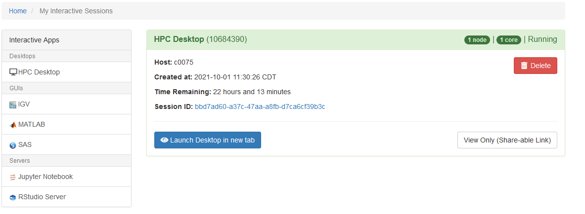
There will be basic information about the number of cores and nodes as well as the job ID in the top part of the job card. The amount of time remaining in the job is included in the card as well as a quick link to the file browser in the Session ID field. Click Launch Desktop in new tab to open your interactive VNC session.

Note

For HPC Desktop, you do not need to request resources after you open the Desktop. You are already on a compute node. Any tasks you run will use the resources you requested when initializing the job.

Note

You can request another interactive session in a terminal in HPC Desktop. Only the terminal you requested the other interactive session in will have access to the new resources. Everything else in the HPC Desktop will run with the resources you requested when creating the initial job.

These interactive jobs can be stopped early by clicking Delete on the right side of the job card.

Standalone Programs

As shown earlier, some software can be run outside of the VNC session. Setup for most of these follow the same rules as creation of an HPC Desktop job in terms of requesting resources. You will also need to select the version of software to use for the job.

Note

Versions in OOD and versions seen when loading modules in a terminal may not match. If you need a specific version available in OOD, submit a support ticket at support@listserv.uab.edu

Jupyter

Jupyter notebooks are available for use in OOD, but some extra setup is required. The extra fields you need to fill out are seen below:

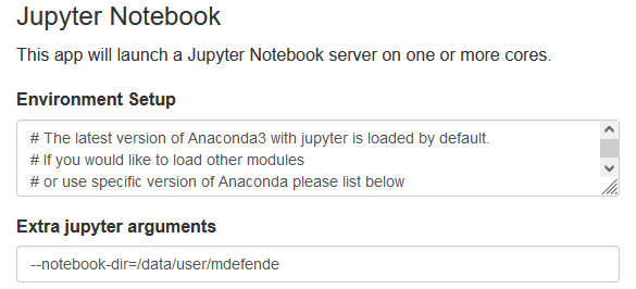
At the bottom of the Environment Setup field, you will need to place a module load command to load the version of Anaconda your Jupyter job will be running. View the list of Anaconda modules installed on Cheaha in a terminal session using module spider Anaconda.

In addition, if you are using the CUDA cores for GPU-enabled machine learning, you will need to load the corresponding CUDA module here. Use module spider cuda to view the list of CUDA modules.

In the Extra Jupyter Arguments field, you will need to add a path to the directory with your jupyter notebooks. For instance, if your notebooks are stored in your user directory, put --notebook-dir=$USER_DATA in this field. You will be able to navigate to the notebook if it is in a subdirectory of notebook-dir.

Submitting the job will bring you to the My Interactive Jobs window while the Jupyter job is initialized. Click Connect to Jupyter to open the Jupyter Home Page.

Note

If you get a Failed to Connect message when opening the job, close the tab and wait a couple of minutes. Jupyter is still initializing and takes some time after the job first begins running.

The Jupyter Home Page will look like:

From here, you can navigate to and select an existing notebook, or you can create a new one using one of your existing virtual environments or the base environment.

Python Libraries and Virtual Environments

To run Jupyter with specific libraries and packages outside of the base install, you will need to create a virtual environment first. You can do this either in an HPC Desktop job or in the Conda tab of the Jupyter homepage.

The Conda has the following layout:

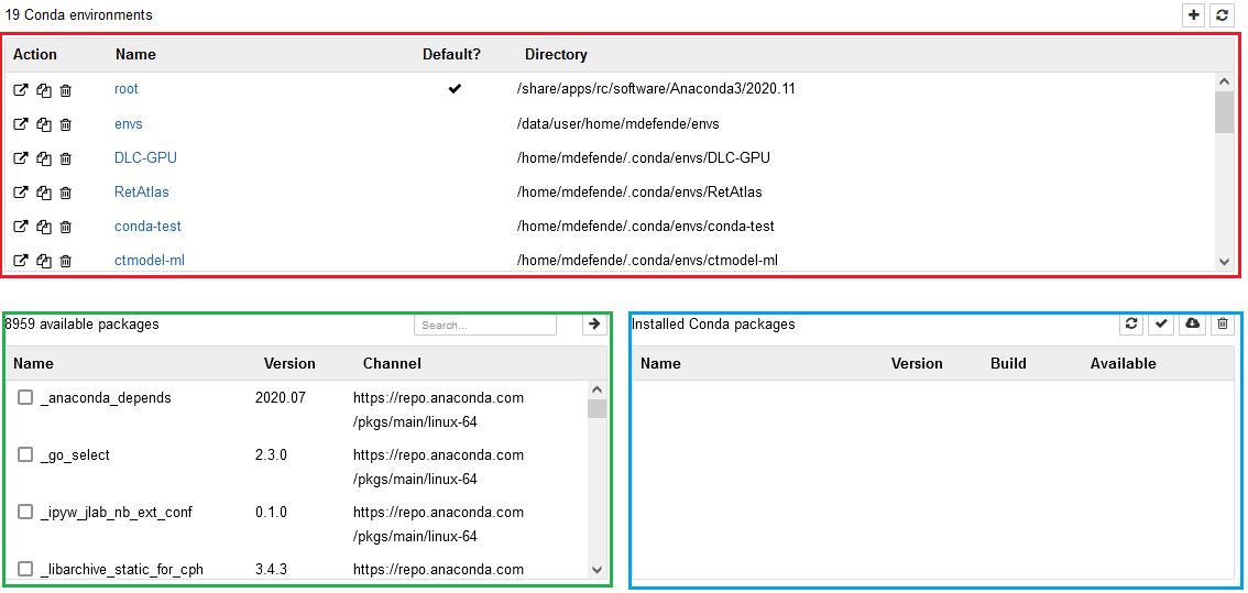
1. Current environments (red): a listing of the current existing environments in your $USER_HOME/.conda/envs folder. 2. Available packages (green): a list of all packages available to install from conda sources. 3. Installed packages (blue): a list of the packages installed in the currently selected environment.

To create a new environment, click the + button at the top of the Current environments pane and enter the name of the environment. After it has been created, you can select packages to install by searching for the package name at the top right of the Available packages pane. After selecting the package, click the -> button, and the package and all its dependencies will be installed.

Note

If a package is not available using the conda command directly, it will not be listed as an available package. Use a terminal window to install the package as necessary.

Note

In order to use an environment with Jupyter, the ipykernel library is necessary. Creating an environment in the Conda tab will autoinstall this library. If using the terminal, use conda install ipykernel to install it.

After successfully creating your environment, navigate to the Files tab. You can create a new notebook using the New dropdown menu in the top right. Select your virtual environment of choice, and a notebook will be created and opened.